
 On Accurate Differential Measurements with Electrochemical Impedance Spectroscopy
S.Kernbach, I.Kuksin, O.Kernbach
Cybertronica Research, Research Center of Advanced Robotics and Environmental Science,
Melunerstr. 40, 70569 Stuttgart, Germany
serge.kernbach@cybertronica.co, igor.kuksin@cybertronica.co, olga.kernbach@cybertronica.co
Received May 15, 2016; Revised August 2, 2016; Accepted September 1, 2016; Published: May 26, 2017;
Available online: June 5, 2017
Abstract
This paper describes the impedance spectroscopy adapted for analysis of small electrochemical changes in fluids. To increase accuracy of measurements the differential approach with temperature stabilization of fluid samples and electronics is used. The impedance analysis is performed by the single point DFT, signal correlation, calculation of RMS amplitudes and interference phase shift. For test purposes the samples of liquids and colloids are treated by fully shielded electromagnetic generators and passive cone-shaped structures. Fluidic samples collected from different geological locations are also analysed. In all tested cases we obtained different results for impacted and non-impacted samples, moreover, a degradation of electrochemical stability after treatment is observed. This method is used in laboratory analysis of weak emissions and ensures a high repeatability of results.
Introduction
Electrochemical impedance spectroscopy (EIS) is a common laboratory technique in analytical chemistry [Chang and Park, 2010], in biological research [Ganesh et al., 2008], for example, in the analysis of DNA or structure of tissues, the analysis of surface properties and control of materials [Macdonald, 2006]. This method consists in applying a small AC voltage into a test system and registering a flowing current. Based on the voltage and current ratios, the electrical impedance Z(ƒ) for a harmonic signal of frequency ƒ is calculated. Measured data are fitted to the model of the considered system and allow identification of a number of physical and chemical parameters.
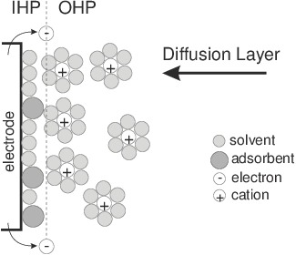
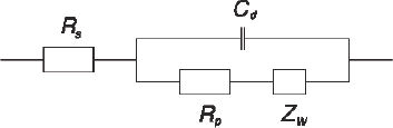
There are several electrochemical models for EIS. In a number of publications (e.g. [Chang and Park, 2010]) a current flowing through the electrode surface is described by the electrochemical reaction O+ne=R,(1) where n is a number of transferred electrons, O – oxidant, R – reductant. The charge transfer through the electrode surface has Faraday and non-Faraday components. Faraday components appear due to transfer of electrons through the activation barrier and are entered into the model as the polarization resistance Rp and solution resistance Rs. Non-Faraday current appears due to charge of capacitor on electric double layers close to electrodes. The mass transport of reactants and products causes so-called Warburg impedance Zw [Chang and Park, 2010], see Fig.1.
The state of the art literature describes changes of physico-chemical parameters of solutions, expressed by Rp, Rs, Cd and Zw, impacted by weak emissions. Sources of such emissions are fully shielded EM (e.g. magnetic vector potential [Puthoff, 1998, Akimov et al., 1992], static electric fields [Burgin, 2008], LEDs/lasers [Kernbach, 2013c]) generators, passive geometrical structures [Kumar et al., 2005], [Mjkin et al., 2002], specific geological locations or other phenomena [Dunne and Jahn, 1995], [Schmidt, 1971], [Tompkins and Bird, 1973]. For instance [Bobrov, 1997], [Bobrov, 2006], [Cardella et al., 2001] investigated the changes of diffusion Gouy-Chapman layer due to a spatial polarization of water dipoles, see also [Stenschke, 1985], [Gruen and Marcelja, 1983], [Belaya et al., 1987]. Appropriate electrokinetic phenomena are described by the Gouy-Chapman-Stern model [Belaya et al., 1987], [Lyklema, 2005]. Papers [Sokolova, 2002], [Andriasheva, 2015] provided data on the conductivity variation of fluids and plant tissues, measured by the conductometric approach with different frequencies. A number of sources [Krasnobrygev and Kurick, 2010], [Krinker, 2012], [Krinker et al., 2012] indicated a change in the of ion transfer of solutions and their detection by potentiometric methods [Kernbach, 2014], [Kernbach and Kernbach, 2014], [Kernbach and Kernbach, 2015]. Measurement of various parameters of chemical reactions exposed to weak emissions is well described, for instance, oxidation of a hydroquinone solution and recording the differential absorption spectrum [Anosov and Truchan, 2003], acetic anhydride hydration reaction and recording the optical density of the solution [Tkachuk et al., 2010], VIS-UV spectroscopy of the acid-base bromothymol indicator and the salt solution SnCl2 [Mjkin et al., 2002].
[a]
[b]
Figure 1: (a) Schematic representation of cations, electrons, molecules and adsorbent solutions on the surface of negatively charged electrode, IHP / OHP – internal and external Hemholtz levels, image from [Chang and Park, 2010]; (b) idealized circuit diagram for the EIS from (a) by following Randles [Randles, 1947]. High-frequency components are shown on the left, low frequency components – on the right; Cd – capacitor on the electric double layer, Rp – polarization resistance; Rs – solution resistance, Zw – Warburg impedance.
Performing multiple measurements of weak emissions by conductometric and potentiometric methods [Kernbach, 2013c], [Kernbach and Kernbach, 2014], [Kernbach and Kernbach, 2015], we discovered a certain specificity of these measurements. In particular this concerns very small changes of measured values, such as a high impact of environmental factors, primarily temperature and appearance of phenomena that are not observed in other areas. These works lead to development of new sensitive measuring devices with differential circuits, ultra-low noise, and thermal stabilization of electronics and samples.
In this paper we describe an adapted EIS approach applied to several test systems. Two different EIS-meters are used. The first one is the developed differential EIS-meter with phase-amplitude detection of excitation and response signals, where the frequency response is analyzed by a single point DFT and correlation analysis. This system is implemented in hardware in the system-on-chip. The second impedance spectrometer is based on the AD5933 chips from Analog Devices and is used as a control device. It supports only DFT with the Hanning window function. Experiments have shown that changes in samples exposed by weak emissions from fully shielded EM generators, passive geometrical structures and geobiological factors are characterized by four values: the differential signal amplitude (this value is included in all amplitude characteristics obtained by the frequency response analysis); the interference phase shift; ratio between imaginary and real parts of the impedance (as shown e.g. by the Nyquist plot) and a variation of electrochemical stationary of samples. It is assumed that these parameters can indicate changes in near-electrode layers and diffusion processes in the Randles electrochemical model [Randles, 1947]. EIS allows analyzing various liquid and colloidal system and, as an example, we perform analysis of bottled water and milk. Since this work has an explorative character, we do not intend to collect statically significant data for a particular system – this represents a task for further works.
This paper has the following structure. The section 2 briefly describes background of EIS, systematic and random errors and used devices. Sections 3 and 4 consider the obtained results and draw conclusions from these measurements.
Impedance Measurement, Errors and Description of the Device
There exists an extensive literature on the EIS, both for theory and models, and for technical aspects of measurements. One of the most common methods for measuring impedances is related to an auto-balancing bridge [Agilent Technologies, 2013], where a test system is excited by the voltage Vv. The flowing current I is converted into a voltage VI by a transimpedance amplifier (TIA). There are several ways how the signals VI and Vv are digitized and processed in further analysis.
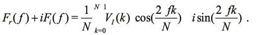
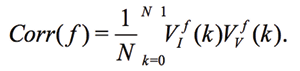
A common approach consists in analyzing the frequency response (frequency response analysis – FRA) of the VI signal, which is based on the discrete Fourier transform (DFT) [Norouzi et al., 2011] and synthesis of ideal frequencies. This method is sometimes called as the single point DFT [Chabowski et al., 2015], [Kim et al., 2005] and requires a fast ADC with 1 msps and more for digitizing the signal VI. The digitized time signal VI(k) with N samples is converted to a frequency signal F(ƒ) containing real Fr(ƒ) and imaginary Fi(ƒ)parts:
 (2)
(2)
It is common to replace w=2pf and to skip ![]() , however these parameters are important for calculating the period [Matsiev, 2015]. The magnitude M(ƒ) and phase P(ƒ) are calculated as:
, however these parameters are important for calculating the period [Matsiev, 2015]. The magnitude M(ƒ) and phase P(ƒ) are calculated as:
 (3)
(3)
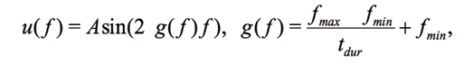
Calculation of (3) is repeated for all ƒ between minimal ƒmin and maximal ƒmax frequencies with the step Δf DFT and FRA differ in the way how basic vectors cos() and sin() are calculated. In the FRA they are synthesized (for example the sine, see [Kim et al., 2005]):
 (4)
(4)
where A is the maximal amplitude, tdur – the duration of the measurement, 0<t<tdur . The synthesized frequency of base vectors must exactly coincide with the frequency of measured signal. In a sense, the expression (2) calculates a correlation between ideal and measured signals. If Vv and VI are digitized strictly at the same time points, for example, by using two synchronous ADCs, and since Vv is a sine/cosine signal, (2) takes the form of correlation between  and
and  (defined for the frequency ƒ)
 (5)
(5)
Expression (5) is more preferable because here a non-harmonic signal of high frequency can be used for synthesizing the Vv.
The literature discusses non-harmonic signals for driving the electrochemical system, for example, [Ojarand and Min, 2013], [Mejнa-Aguilar and Pallas-Areny, 2009] used digital square waves. An excitation by a broadband noise signal is utilized for a fast impedance spectroscopy [Smith, 1976]. The analysis can be carried out with a direct amplitude and phase detection. For instance, the maximal or RMS amplitude of VI as well as a phase shift between Vv and VI can be calculated without FRA. In more complex cases, the Laplace transform is performed between Vv and VI.
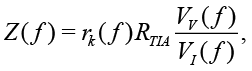
If the magnitude or the RMS amplitude of Vv and VI are known, the impedance Z for the auto-balancing method is defined as
 (6)
(6)
where RTIA is a reference resistor in TIA, rk(ƒ) is a frequency-dependent gain caused by analog circuits, inaccuracies in discrete elements, etc. [Agilent Technologies, 2013]. Thus, Z is inversely proportional to VI.
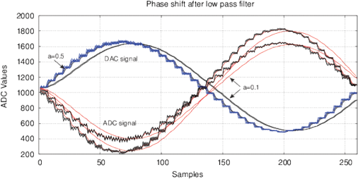
Performing measurements, we found an interesting effect of changing the phase of differential signal (Vv–VI), as shown in Figs. 11(b), 14(b). This unexpected result is not shown by the phase analysis with FRA (3). This phase variation is created by a combination of two factors: the use of direct digital synthesis (DDS) with a low number of samples and application of the digital infinite impulse response filter (IIR filter):
 (7)
(7)
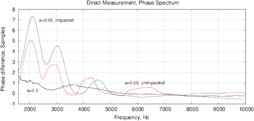
where xn are discrete samples of an input signal, yn is the filtered signal, a is a coefficient. Figure 2 shows the use of a filter for one period of DDS signal with 40 samples and the frequency spectrum up to 10 kHz.
[a]
[b]
Figure 2: The effect of phase variation after applying the digital IIR filter (7) with a=0.5, a=0.1 and a=0.05 and for a DDS signal synthesis with a small number of samples for (a) one signal period with 40 samples, 3 kHz; (b) the frequency spectrum up to 10 kHz.
Such DDS synthesis includes high frequency components (up to 400-600 kHz) in a low frequency signal. Both low- and high-frequency components impact the samples, this is similar to using a broadband noise for a fast spectroscopy [Smith, 1976]. The IIR filter at a<0.5 increases the delayed term yn-1, however it appears differently at different frequencies. Thus, we assume that the main reason for the periodic phase shift is an interference with the high-frequency components in the DDS signal. Hereinafter, this parameter will be referred to as an interference phase shift Φ. Treatment of samples modifies the response to high frequency components, which is manifested as a variation of Φ. With increasing the frequency, this effect decreases, we observe also a smaller variation of Φ(ƒ).
As emphasized in [Chang and Park, 2010], FRA can only be used for stable and reversible systems in dynamic equilibrium, thereby the linearity and stability of electrochemical system should be provided. These are so-called steady-state conditions, whereby deviations from them can appear, for example, in the form of long transient processes. The stationarity is usually not investigated by impedance spectroscopy, but it can represent an additional source of information about the electrochemical processes before and after the treatment of samples.
The measurement approach for weak emissions is described in [Kernbach and Kernbach, 2015], [Kernbach, 2013b], [Kernbach and Kernbach, 2014]. It uses two identical channel A (experimental) and B (control), which apply the same exciting signal Vv . Spectrograms A and B are subtracted from each other, the resulting difference spectrum is close to zero at all frequencies if the samples A and B are equal. A non-zero differential spectrum indicates differences in samples. Since both samples are prepared at the same temperature, in the same EM, light and other conditions, the difference is caused only by exposure to experimental factors. This method requires at least two measurements. In the first one the samples A and B are measured before impact, these data are used for calibration. The second measurement of A and B is performed after exposing the sample A. The measurement result consists of two differential curves: the calibration (close to zero) and experimental ones. The difference between them allows making conclusions about impact on the sample A.
The Error Analysis
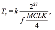
EIS has several systematic and random errors. The first systematic error is related to the period and phase of synthesized base vectors and measured signal. The period of signals accumulated in arrays Vv and VI must be expressed by an integer. If this condition is not met, so-called leakage errors occur. This problem is solved in three ways [L.Matsiev, 2015]. Firstly, it is proposed to select the sweep frequencies ƒ in such a way that VI always contains an integer number of period k. The paper [Chabowski et al., 2015] considered a choice of ƒ based on
 (8)
(8)
where Ts is the digitization time, MCLK is the fundamental frequency of AD5933 ([Chabowski et~al., 2015] is written in the context of this scheme). The obvious drawback of this approach is that the frequency step Δƒ is large and it is impossible to perform a detailed frequency scan of the test system.
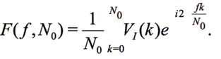
The second method is based on adapting the number of samplings N at each sweep. The number of samples N in VI is changed to N0 in (2) so that exactly one period of VI is stored at each reading:
 (9)
(9)
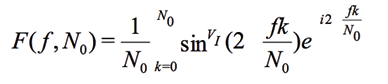
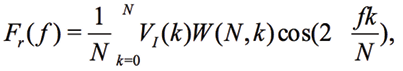
Since the base vectors at FRA must have the same frequency as VI, which is a response to the excitation signal sin() in Vv (written as sinVI() ), this leads to
 (10)
(10)
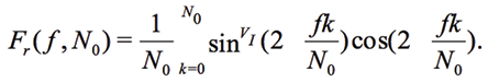
or components-wise, e.g. for the real part of Fr
 (11)
(11)
Since we record only one period of signal, N0=ƒ(ƒ) is valid for all frequencies and the main variation of Fr(ƒ(ƒ) occurs due to N0
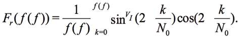 (12)
(12)
Despite ƒ is disappeared from sin() and cos(), VI and Vv are still affected by the test system at frequencies ƒ. Therefore, the physical meaning of (12) consists in analysis of amplitude variation, phase and waveform of VI at the frequency ƒ. The disadvantage of this method lies in the rapid decrease of N0 when increasing the frequency ƒ. Figure 3 shows the relationship between ƒ and the number of samples N0 by selecting a different number of periods in the VI array. Thus, it is necessary to introduce the measurement ranges with a different number of periods.
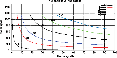
Figure 3: The relationship between the frequency ƒ and the number of samples N0 by selecting a different number of periods in VI.
The third approach consists in introducing so-called window function W(N,k)
 (13)
(13)
which modulates the signal VI and reduces its amplitude to boundaries of window with N samples. The AD5933 uses the Hanning function [L.Matsiev, 2015]:
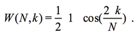 (14)
(14)
The functions (13) allows keeping N at the same level for all frequencies, which is useful for digitizing the signal. However, this method distorts the original signal, instead of VI(k) the signal VI(k)W(N,k) is analyzed. This problem is discussed in literature [Harris, 1978]. Consequences of using (13) is reflected in Fig. 9 as an appearance of new periodic components that are not present in the original signal.
The second source of error is the frequency characteristics, and especially the limited bandwidth of analog components. As a result, the magnitude of VI decreases with ƒ and the magnitude of the impedance  increases. The problem of increasing impedance exists in all EIS-meters, which solve it in different ways. For example, AD5933 requires two-point or multi-point calibration [Devices, 2013] (see Section 2.4).
The third source of systematic error represents a small number of samples for DDS synthesis of Vv when measuring the test system with a large capacitive component. This leads to peaks in VI and significantly increases noise, a detailed examination of this effect for AD5933 is given in [Chabowski et al., 2015].
The impedance Z of test system and the reference resistance RTIA in TIA should be similar
Z ~RTIA, (15)
otherwise the TIA can become saturated and the signal VI is significantly distorted. Systematic errors are also influenced by the electrode polarization, which is a well-known problem of impedance spectroscopy [Ishai et al., 2013], [Kalvoy et al., 2011], especially at low frequencies. This effect is markedly manifested when using small-sized electrode and highly conductive liquids.
Random error also has several components. Firstly, a noise introduces a small random error of detecting the phase-amplitude characteristics of Vv and VI. Secondly, the EIS measurement interacts with samples due to the applied voltage and flowing current. When conducting multiple repeat measurements with the same sample, the measured parameters can “float” – that introduces an additional error. A large random error occurs at variation of initial conditions for measurements. This includes small changes in the cell constant temperature variations of containers and the liquid preparation. These small variations between control and experimental samples are well measurable by the exact differential method and can lead to wrong conclusions about the impacted fluid.
The EIS Device
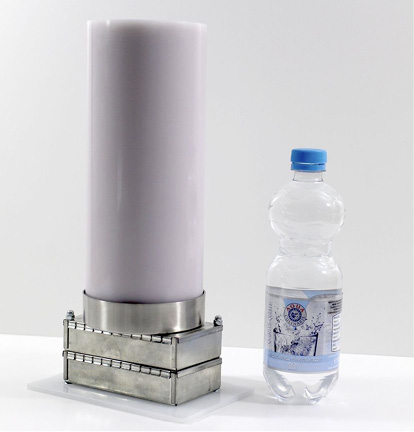
Measurement of weak emissions requires differential measurement circuits and ther-mal stabilization of system and samples. Available commercial EIS-meters do not offer these options. In the previous works we used commercial conductivity meters, the pH and Redox meters [Kernbach and Kernbach, 2014]. However they did not provide accurate enough measurements, allowing to characterize weak emissions. In this work we decided to adapt the MU system [Kernbach and Kernbach, 2014], [Kernbach and Kernbach, 2015] for EIS measurements with necessary methodology and metrology, and also to use available devices for control measurements. The first versions of MU-EIS on the PSoC (Programmable System on Chip) architecture were developed in 2012 [Kernbach, 2013c], [Kernbach, 2013a] and 2013 [Kernbach, 2013b], [Kernbach and Kernbach, 2016] as devices for DC and non-contact high-frequency conductometry. The MU-EIS meter, see Fig. 4, supports differential measurements and temperature control, the digital signal processing (DSP core) is implemented in hardware on reconfigurable PSoC architecture.
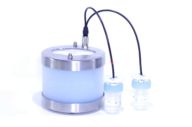
Figure 4: Differential impedance spectrometer on MU-EIS system with temperature stabilization of samples and electronic components.
The scheme AD5933 [Devices, 2013] has been selected as a commercially available solution. It is a precision impedance spectrometer on a single chip, which has an internal DSP core and is connected to the host system by I2C interface. There are a large number of available devices based on this scheme [Chabowski et al., 2015], [Ghaffari et al., 2015], [Hoja and Lentka, 2010]. The termostabilization was performed by the MU system, two identical AD5933 boards are used for differential EIS-meter, see Fig. 5. Software provided by Analog Devices was rewritten in order to support differential functions.
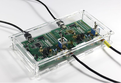
Figure 5: Differential impedance spectrometer on AD5933.
In general, both EIS-meters are similar. Synthesis of the signal Vv occurs by DDS (AD5933 – 27-bit frequency resolution, MU-EIS – 32 bits), the I–V conversion is performed by TIA, the signals are digitalized by 12 bit 1 MSPS SAR ADC (MU-EIS uses two synchronous 1.2 MSPS SAR ADCs for simultaneous sampling of Vv and VI signals). For impedance matching, both systems use external analog circuitry. There are several fundamental differences between the versions. AD5933 uses the Hanning window function, the number of samples N is fixed on 1024 and the system allows only 512 frequencies ƒN within 5 frequency bands, the system allows any number of scanning frequencies. Also, the upper frequency limit in the MU-EIS is 0.6MHz, while the AD5933 is limited by 0.1MHz. MU-EIS allows using non-harmonic signals Vv for driving an electrochemical system, while FRA of the AD5933 does not permit this.
In both cases the meter is connected to two measurement cells with 15 ml containers. Electrodes (graphite, platinum or stainless steel) are mounted in the upper part of measuring containers, see Fig. 6.
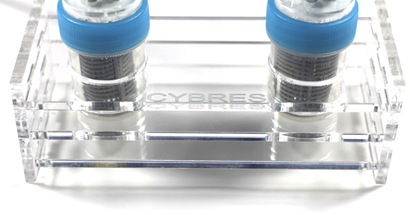
Figure 6: Measurement cells with 15 ml containers.
Emitting Devices
The device “Cosma” shown in Fig. 7(a) was used to prepare the water samples. This device consists of three subsystems that can be switched on or off: LED emitters of ultrashort pulses (based on [Bobrov, 2006], [Kernbach, 2013c], [Kernbach, 2013a], the needle emitter of electrostatic field (based on [Weinik, 1981], [Weinik, 1991], [Chigewskij, 1973], [Chigewskij, 1930]) and the generator of AC magnetic field (based on [Anosov and Truchan, 2003], [Dulnev, 2004], [Asheulow et al., 2000], [Britova et al., 1998]). The generated emission is modulated between 0.1 Hz and 1 kHz. The device also includes a camera for installing a donor substance in order to investigate the imprinting effects [Kernbach, 2015]. For shielding purposes, emitting elements and electronics are enclosed into grounded metal boxes in the lower part.
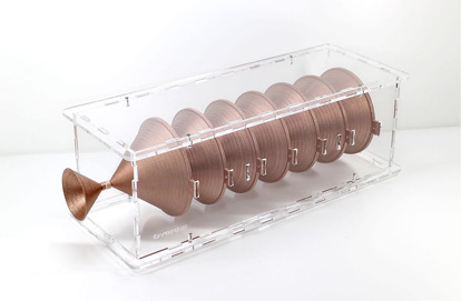
A fully passive generator “Contur” is represented by a system of cone-shaped geometrical forms, see Fig. 7(b). Each cone is made from organic polymer coated from both sides by a copper, each polymer/copper layer is at least of 0.3mm thick. Cones are placed into each other so that a top of the next cone enters into the previous cone on 1/3 or 1/2 of its height or lies on the baseline. This placement is denoted as the focus position. Experiments are performed with 0%, 33% and 50% focus position and with systems of 3, 4, 5, and 7 cones.
[a]
[b]
Figure 7: (a) Prototype of the “Cosma” device used for preparation of liquid samples, suspensions and gels; (b) The system “Contur” of passive cone-shaped geometrical structures.
Calibration
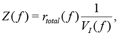
Calibration of EIS is required to determine the overall gain and to remove nonlinearity and errors introduced by analog components, connecting wires and electrodes. Moreover, a special calibration fluid is required for measuring the cell constant. Attention should be paid to two important points expressed by (6): firstly, the impedance Z is inversely proportional to VI, secondly, FRA magnitude of Vv is a constant. This allows rewriting (6) in the form
 (16)
(16)
where rtotal(ƒ) is defined by calibration. Another approach consists in calculating the RMS values  ,
, 
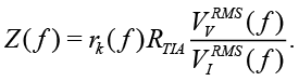 (17)
(17)
Since the value of RTIA is known, the expression (17) allows auto-calibration for all measured frequencies ƒ with accuracy of rk(ƒ). During calibration and measurements it is necessary to set the amplitude of Vv so that the amplitude VI remains within the operational range of ADC and TIA.
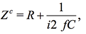
For calibration it is convenient to use the resistor R and the capacitor C. The impedance ZC for a serial connection of R and C is expressed as
 (18)
(18)
where 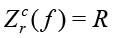 and
and 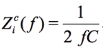 . For example, the impedance of the 10nF capacitor at the frequency of 1 kHz is equal to 15915.5Ohm. If the Zm(ƒ) is the measured impedance at the frequency ƒ for R and C, the arrays Kr(ƒ) and Ki(ƒ), represented in the form of
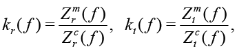 (19)
(19)
will contain the calibration coefficients of imaginary and real parts for each frequency. For AD5933 [Analog Devices, 2013] the gain G for calibration impedance Zc is calculated as
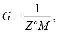 (20)
(20)
where M is the magnitude (3). Each measured impedance Z is adjusted by G in the form of
 (21)
(21)
Figure 9 shows the real and imaginary parts of FRA, as well as the magnitude and phase of the impedance with the calibration resistance of 17.6 kOm. As mentioned above, AD5933 circuit utilizes a window function, the oscillating components of sin() and cos() are well visible in the output arrays Re(z) and Im(Z), see the Nyquist plot in Fig. 8. To compensate this effect, AD5933 requires a calibration across all frequencies, indicating RC models of the calibrated device.
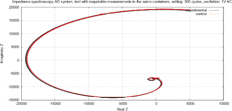
Figure 8: The Nyquist plot Re(Z) of Im(Z) for AD5933, oscillating components due to Hanning window function are clearly visible.
[a]
[b]
[c]
[d]
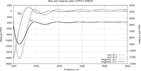
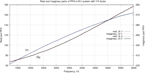
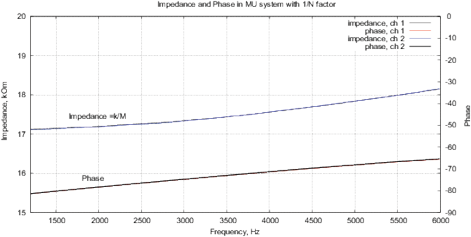
Figure 9: (a) Real and imaginary parts and (b) impedance and phase of the FRA obtained for the AD5933; (c) real and imaginary parts and (d) impedance and phase of the FRA obtained with MU-EIS. The measurements were performed with a resistance of 17.6 ohms in steps of 10 Hz with single-point calibration, excitation is performed by a sinusoidal signal.
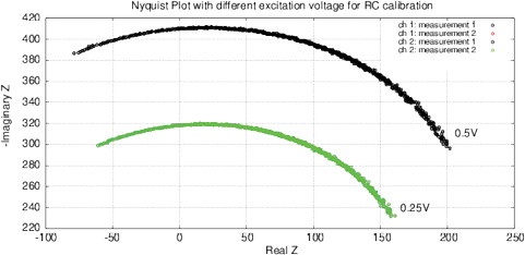
Figures 9(d,c) show results the real and imaginary parts of FRA for MU-EIS as well as the magnitude and phase without oscillations. Phase is about –90º because of TIA converter. The correlation curve is obtained by (5), it follows the magnitude. Figure 10 shows the calibration data for the single-point calibration with R=17.6 kOm, C=10nF and the obtained Nyquist plot for Re(Z) and Im(Z).
[a]
[b]
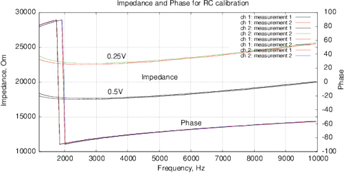
Figure 10: (a) Nyquist plot and (b) impedance and phase for the calibration RC-chain (17.6 kOm, 10 nF) with a one-point calibration. Phase jump is due to the function tan 1( ) in (3).
[a]
[b]
Figure 11: Control measurements of the bottled water “Black Forest,” see description in text. (a) The differential amplitude spectrum VI, obtained by MU-EIS; (b) differential phase spectrum by the MU-EIS.
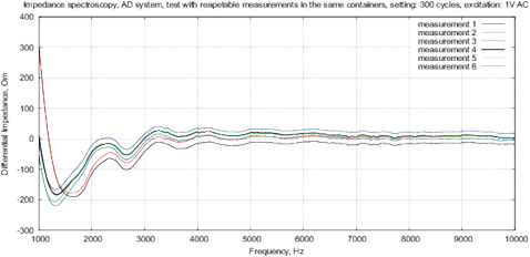
Figure 12: Control measurements of the bottled water “Black Forest” with AD5933, differential impedance spectrum, see description in text.
The paper [Kernbach and Kernbach, 2015] expressed arguments against the calibration of differential measurements because the expressions (19) and (20) introduce additional noise from test measurements. Since the amplitude of differential signal is small, this noise complicates a detection of small changes. For this reason, Section 3 shows the results without calibration.
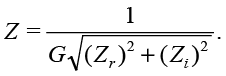
The cell constant includes factors associated with the geometry of measuring cell and electrodes, the surface area, fluid dynamics in the cell, etc. To analyze the errors caused by variation of the cell constant, the following method is used [Kalvoy et al., 2011]. First, each measurement starts from dry electrodes and is repeated to determine the reproducibility of measurements. Further, the electrodes are removed and dried. This measurement cycle is repeated again to determine the degree of variability. Figures 11 and 12 show an example of such measurements with 10 iterations both for MU-EIS, and for AD5933. Results for the same initial conditions do not vary more than ±0.1 ohms (0.001% of the total value). The variation of initial conditions is between ±5 Ohm to ±20% Ohm (from ±0.05% to ±0.2% of full scale).
Measurement Results
The experiments are performed in the following way. The bottled water “Black Forest” at room temperature is poured into four 15 ml containers (two samples A and B) for AD5933 and MU-EIS system. Samples thermostat is set on 27ºC. The containers are kept in thermostat for 20 minutes to equalize the temperature before starting measurements.
1. First test measurements are performed with A and B samples at frequencies between 1 kHz and 10 kHz with 10 Hz steps. Sweeps are repeated 10 times, the spectra of A and B are subtracted from each other, as a result 10 differential spectral curves are obtained. The purpose of this test is to assess the bias error of repeating measurements.
2. To determine the random error, the samples are removed from the thermostat and put on a shelf. After 30 minutes the samples are placed again in the thermostat and 10 differential measurements as described in (1) are performed.
3. The samples A and B are removed from the thermostat, the sample A is treated by “Cosma” or “Contur” devices. After this, the sample A is rested about 10 minutes, then measurements with both samples are performed again.
4. To determine the random error after exposure, the samples (after exposure of the sample A) are removed from the thermostat, rested for 30 minutes, and then 10 differential measurements are carried out.
Thus, this approach allows evaluating the variations of systematic and random errors as well as to estimate the effect of exposing the water to experimental factors. In total, 5 series of experiments with multiple iterations are performed.

Figure 13: Setup with cone-shaped geometric structures and water samples.
[a]
[b]
[c]
[d]
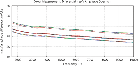
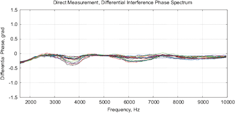
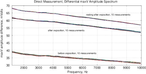
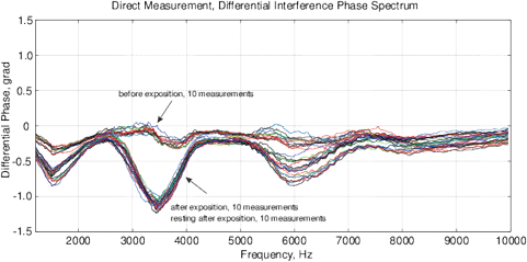
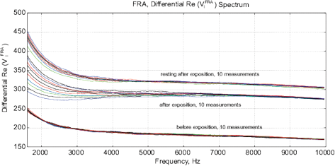
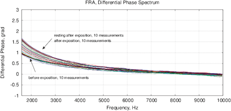
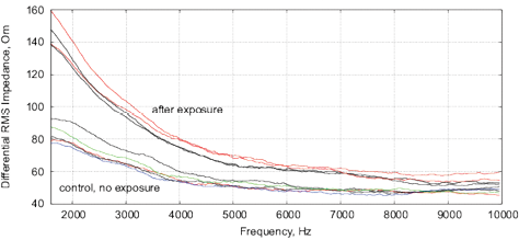
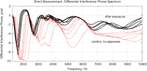
Figure 14: The experimental results with water exposed in the “Cosma” generator, excitation time before measurement is 1 ms, the MU-EIS system is used. (a,b) Direct measurements of amplitude and phase characteristics, (c,d) Results of frequency response analysis.
[a]
[b]
[c]
[d]
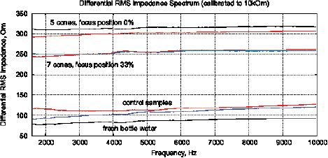
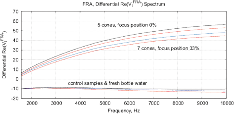
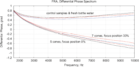
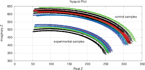
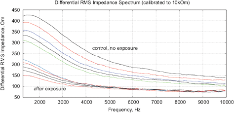
Figure 15: The results of EIS analysis of water samples placed in front of passive cone-shaped geometric structures with focus position of 0% and 33%. (a) Differential RMS impedance (calibrated to 10k), (b) FRA, the differential spectrum of Re(V1)impedance, (c) FRA, differential phase spectrum, (d) the Nyquist plot. Thermostat temperature was set to 28°C±0.02°C.
[a]
[b]
[c]
[d]
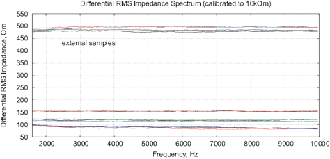
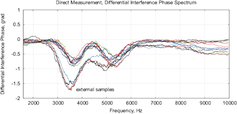
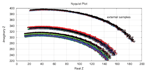
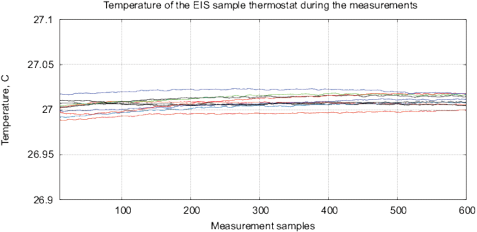
Figure 16: The results of EIS analysis of 4 water samples placed for 12 hours in different locations, the “external sample” – the water sample placed in the far room (2.5 km from the lab) that shows a strong deviation of the measured EIS parameters, each measurement is repeated twice. (a) Differential range RMS impedance (calibrated to 10k), (b) the differential spectrum of the interference phase shift, (c) the Nyquist plot, (d) thermostat temperature with samples during the measurement (the set temperature is 27°C).
Experimental Series 1. Figure 11 shows the results of one of the control experiments with the procedure (1). The amplitude and phase characteristics show small changes caused by variation of initial conditions. These experiments are repeated more than 20 times.
Experimental Series 2. This series has several dozen of iterations, where various parameters of the module “Cosma” are tested. The results of one of these experiments is shown in Fig. 14, where the procedures (2) and (3) are applied – water samples are exposed and the random error is estimated after the exposure. The exposition time varies between 10 and 30 minutes. The variation of random error before and after the exposure has a similar character. However, significant changes are observed in the exposed samples. The measurement results can be characterized by  – amplitude changes of the differential signal Re(V1FRA), Re(Z), M(f), Corr(ƒ) exhibit similar changes), ΔΦ – change of the interference phase shift and
  – variation of stationary conditions. Repeated measurements of the irradiated samples after 6-24 hours show a strong variation at low frequencies that can indicate a change of electrochemical stability.
Experimental Series 3. These experi-ments are conducted with the cone-shaped geometric structures. Containers with water are placed in front of the output cone for 36 hours, see Fig. 13. Control measurements are performed with fresh bottle water as well as with control containers rested for 36 hours without any impact. Results of several measurements are shown in Fig. 15. There are almost no differences between control samples and fresh bottle water, however, an essential difference between experimental and control samples. Since all containers are positioned in one room with the same EM and other environmental factors, we can assume a non-electromagnetic impacting factor related to the shape effect.
Experimental Series 4. For this series, four identical samples of water in 15ml containers are placed for 12 hours in different locations with the distance between 3 meters up to 2.5 km from each other. This experiment is repeated 4 times. Fig. 16 shows the EIS results for one of the experiments. In addition, it shows the temperature of samples during measurements, the temperature fluctuations do not exceed 0.02°C. The “external sample” (sample from the far location) demonstrates the largest changes of EIS parameters. Since the measured values of EM and radiation background in these locations are on the same level and conform to the EC/DIN norms, we can explain the EIS differences of samples only by some geological or geo-biological factor.
Experimental Series 5. This series of experiments is motivated by the works of V.A.Sokolova’s group [Sokolova, 2002], where a gel-like consistency of milk exposed by the A.Deev’s generator was achieved. Moreover, the well-known patents of R.Pavlita [Foundation, 1992], A.Deev’s work [May et al., 2014] and ISTC VENT (group of A.E.Akimov) [Kernbach, 2013] indicated a capability of cleaning suspended solutions exposed to some sources of weak emissions. For example, Fig. 17 shows samples of milk two weeks after irradiation in the module “Cosma,” we indeed observe a difference between experimental and control samples of the clotted milk.
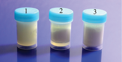
Figure 17: The milk samples two weeks after irradiation, the container 1 has an experimental sample, the containers 2 and 3 – control samples. Clotted milk in the container 1 differs significantly from 2 and 3.
[a]
[b]

[c]
[d]
Figure 18: The results of EIS analysis of milk samples, 5 replicate measurements are shown in each case, (a, c) – the samples immediately after irradiation, (b, d) – the sample 24 hours after irradiation, the samples are stored at room temperature. (a, b) Differential impedance spectrum RMS (calibrated to 10k); (c, d) spectrum of differential interference phase shift. The thermostat temperature is set to 27º C±0.02ºC, as shown in Fig. 16(d).
Experiments are performed with 1.5% milk from different manufacturers and are repeated 4 times. The results are shown in Fig. 17. Similarly to water samples, we observe a change of impedance and interference phase shift of irradiated samples. However, in these experiments, a strong variation of electrochemical stability before, after exposure and 24 hours after exposure is observed. Apparently, the complex organic compounds have their own dynamics, caused by biochemical processes. For example, determining the freshness of milk by measuring its conductivity is well known. In this sense, milk is not a “good EIS marker” for analyzing weak emissions.
Conclusion
This paper demonstrates an accurate differential approach with electrochemical impedance spectroscopy adapted for analysis of weak emissions. This method provides reliable results with a high degree of repeatability. In experiments with samples exposed to artificial and natural EM/non-EM emission, the measurement results allow distinguishing treated and untreated samples in all cases. Due to a short measurement time, this method is potentially suitable for a rapid analysis in field conditions. Other applications, e.g. in autonomous systems [Levi et al., 1999, Eiben et al., 2012], robotics [Kornienko et al., 2005, Kornienko et al., 2001] or industrial manufacturing [Kornienko et al., 2003] are also possible.
The values of  (differential signal amplitude), ΔΦ (interference phase shift), Re(Z), Im(Z) (for example, the Nyquist plot) and changes in electrochemical stationary describe differences between control and experimental samples. To some extent, these value can characterize the exposure by weak emission. Based on the Randles’ electrochemical model [Randles, 1947], as shown in Fig. 1, these parameters indicate a change in the near-electrode layer parameters and diffusion processes associated with Warburg impedance.
Three types of measurements are per-formed: test measurements with the variation of initial conditions, impact by experimental devices, and analysis of samples taken from different geological locations. In all cases, the differential measurements (comparison with control untreated samples) are used and the parameters  , ΔΦ and Re(Z), Im(Z) characterized the impact. Results of impact are more “evident,” if the measurements are performed 12-24 hour after exposition.
The greatest measurement error is caused by the variation of initial conditions and electrochemical stability. Since the EIS is an “invasive” method of analysis, i.e., this method interacts with samples during measurement, not all liquids and not all voltages Vv are suitable for the analysis of weak interactions. It is necessary to find a fluid with a high electrochemical stability and a good response to weak emissions. This liquid will act as an “EIS marker.”
Experiments with commercial devices based on AD5933 showed three major disadvantages: lack of temperature stabilization, the inability of differential measurements and FRA analysis with window functions. The resulting error of such measurements are often higher than the amplitude of measured signals caused by the impact of experimental factors. In particular, oscillations caused by the Hanning function in AD5933 complicate the differential analysis. Similarly to the potentiometry [Kernbach and Kernbach, 2014], [Kernbach and Kernbach, 2015], is necessary to develop instruments specifically adapted for such measurements.
In preparing and conducting the experiments, similar works of other authors are analyzed. In particular publications of pioneers of Soviet unconventional studies V.A.Sokolova et al [Sokolova, 2002] is considered. The well-known publications of A.E.Akimov’ group [Akimov et al., 2001] are also referring to these works. We can confirm that the largest changes in impacted samples relate to amplitude parameters that are measured by Sokolova as a relative dispersion of conductivity. In general terms, we think that the replication of those experiments is successful, however, several issues remained open. For example, the used fluid and organic tissues posses different electrical conductivity. It is not clear how the impedance matching was performed. Sokolova also obtained different conductivity values at frequencies from 1 kHz to 8 kHz for the same material. In our experiments, however, the differences in conductivity are much lower. This might indicate considerable measurement errors in Sokolova’s experiments, e.g. caused by manual insertion of electrodes and missing temperature stabilization.
In further studies we will collect larger statistics for various liquid, suspensions and gels, as well as for methods and devices generating weak emissions.
Discussion with Reviewers
Reviewer 1: “What information can be discovered using this method concerning the structure of water or aqueous solutions?”
There are several issues here. First of all, the differential EIS with thermostabilization of samples provides a great resolution of impedance / conductivity / resistivity measurements – e.g. up to 10-11 S/cm in conductivity of distilled water. The long-term measurement allows charactering the dynamics of impedance, e.g. changes caused by self-ionization, by dissolving of atmospheric CO2, or by exposure of so-called “weak emissions” possessing non-electromagnetic, non-acoustic, non-thermal and non-mechanical nature. This allows a reliable identification and characterization of such weak impacts. Secondly, the measurements demonstrated that electrochemical properties of water can be changed even when the samples are exposed by fully passive geometric objects. It seems that the “structure of water” can be impacted in non-chemical and non-electromagnetic way, currently multiple groups around the world have similar results. The response obtained on different scanning frequencies allows testing several research hypotheses: do these changes point to different properties of Gouy-Shapman layer of exposed/unexposed samples (similar results have been obtained for DC conductometry with very large statistics), to ion-ion/ion-dipole interactions, to changing the self-ionization constant (e.g. by impacting random fluctuations in molecular motions)? EIS spectroscopy can also add some details on dynamics of relationship between resistive and capacitive electrochemical components under non-chemical and non-electromagnetic impacts (e.g. in addition to classical Randles model). In general, this instrument and measurement methodology represent a powerful tool for a deeper understanding, assessing and validating of interactions between the “structure of water” and various natural and artificial weak emissions.
References
[Agilent Technologies, 2013] Agilent Technologie, A. (2013). Agilent Impedance Measurement Handbook. Agilent.
[Analog Devices, 2013] Analog Devices (2005-2013). Data sheet AD5933: 1 MSPS, 12-Bit Impedance Converter, Network Analyzer.
[Akimov et al., 1992] Akimov, A., Tarasenko, V., Samochin, A., Kurick, I., Meiboroda, V., Licharev, V., and Perov, U. (1992). Patent SU1748662 Approach and device for correction of structural properties of materials (rus).
[Akimov et al., 2001] Akimov, A., Tarasenko, V., and Tolmachev, S. (2001). Torsion communication – new system for telecommunication (rus). Electrocommunication, (5).
[Andriasheva, 2015] Andriasheva, M. (2015). Changing water properties through numeric codes (rus). IJUS, 10(3):7–14.
[Anosov and Truchan, 2003] Anosov, V. and Truchan, E. (2003). New approach to impact of weak magnetic fields on living objects (rus). Doklady Akedemii Nauk: biochemistry, biophysics and molecular biology, (392):1–5.
[Asheulow et al., 2000] Asheulow, A., Dobrovolskij, U., and Besulik, V. (2000). Impact of electric and magnetic fields on parameters of semiconductor devices. Technology and design in electronic equipment, (1):33–35.
[Belaya et al., 1987] Belaya, M. L., Feigel’man, M. V., and Levadnyii, V. G. (1987). Structural forces as a result of nonlocal water polarizability. Langmuir, 3(5):648–654.
[Bobrov, 2006] Bobrov, A. (2006). Investigating a field concept of consciousness (rus). Orel, Orel University Publishing.
[Bobrov, 1997] Bobrov, V. (1997). Reaction of double electrical layer on torsion field (rus). In BINITI N 1055-B97.
[Britova et al., 1998] Britova, A., Adamko, I., and Bachurina, V. (1998). Activation of water by laser light, magnetic field or by their combination (rus). Vesnik of Novgorod’s State University, (7).
[Burgin, 2008] Bürgin, L. (2008). Der Urzeit-Code. Herbig.
[Cardella et al., 2001] Cardella, C., de Magistris, L., Florio, E., and Smith, C. (2001). Permanent changes in the physico-chemical properties of water following exposure to resonant circuits. Journal of Scientific Exploration, (15(4)):501–518.
[Chabowski et al., 2015] Chabowski, K., T.Piasecki, A.Dzierka, and Nitsch, K. (2015). Simple wide frequency range impedance meter based on AD5933 integrated circuit. Metrology and Measurement Systems, XXII(1):13–24.
[Chang and Park, 2010] Chang, B.-Y. and Park, S.-M. (2010). Electrochemical impedance spectroscopy. Annu. Rev. Anal. Chem., 3:207–29.
[Chigewskij, 1930] Chigewskij, A. (1930). Epidemiological catastrophes and periodic activity of the Sun. Moscow.
[Chigewskij, 1973] Chigewskij, A. (1973). Electric and magnetic properties of erythrocytes (rus). Moscow.
[Dulnev, 2004] Dulnev, G. (2004). Looking for a new world (rus). Wes.
[Dunne and Jahn, 1995] Dunne, B. J. and Jahn, R. G. (1995). Consciousness and anomalous physical phenomena. Technical Note PEAR 95004.
[Eiben et al., 2012] AE Eiben, Serge Kernbach, Evert Haasdijk (2012). Embodied artificial evolution, Evolutionary Intelligence, Vol. 5, Issue 4, p. 261-272.
[Foundation, 1992] Foundation, T. P. (1992). Note on work of Robert Pavlita and his experiments in bio-energy. www.keelynet.com/biology/pavlita1.txt.
[Ganesh et al., 2008] Ganesh, V., Pandey, R., Malhotra, B., and Lakshminarayanan, V. (2008). Electrochemical characterization of self-assembled monolayers (sams) of thiophenol and aminothiophenols on polycrystalline au: effects of potential cycling and mixed sam formation. J. Electroanal. Chem, 619:87–97.
[Ghaffari et al., 2015] Ghaffari, S., Caron, W.-O., Loubier, M., Rioux, M., Viens, J., Gosselin, B., and Messaddeq, Y. (2015). A wireless multi-sensor dielectric impedance spectroscopy platform. Sensors, 15:23572–23588.
[Gruen and Marcelja, 1983] Gruen, D. W. R. and Marcelja, S. (1983). Spatially varying polarization in water. a model for the electric double layer and the hydration force. J. Chem. Soc., Faraday Trans. 2, 79:225–242.
[Harris, 1978] Harris, F. (1978). On the use of windows for harmonic analysis with the discrete fourier transform. IEEE Proc., 66:51–83.
[Hoja and Lentka, 2010] Hoja, J. and Lentka, G. (2010). Interface circuit for impedance sensors using two specialized single-chip microsystems. Sensors and Actuators A: Physical, 163(1):191 – 197.
[Ishai et al., 2013] Ishai, P. B., Talary, M. S., Caduff, A., Levy, E., and Feldman, Y. (2013). Electrode polarization in dielectric measurements: a review. Measurement Science and Technology, 24(10):102001.
[Kalvoy et al., 2011] Kalvoy, H., Johnsen, G., Martinsen, O., and Grimnes, S. (2011). New method for separation of electrode polarization impedance from measured tissue impedance. The Open Biomedical Engineering Journal, 5:8–13.
[Kernbach and Kernbach, 2014] Kernbach, S. and Kernbach, O. (2014). On precise pH and dpH measurements (rus). International Journal of Unconventional Science, 5(2):83–103.
[Kernbach and Kernbach, 2015] Kernbach, S. and Kernbach, O. (2015). Detection of ultraweak interactions by precision dph approach (rus). IJUS, 9(3):17–41.
[Kernbach and Kernbach, 2016] Kernbach, S. and Kernbach, O. (2016). Impact of structural elements on high frequency non-contact conductometry. IJUS, 12-13(4):47–68.
[Kernbach, 2013a] Kernbach, S. (2013a). Exploration of high-penetrating capability of LED and laser emission. Parts 1 and 2 (rus). Nano- and microsystem’s technics, 6,7:38–46,28–38.
[Kernbach, 2013b] Kernbach, S. (2013b). On metrology of systems operating with “high-penetrating” emission (rus). IJUS, 1(2):76–91.
[Kernbach, 2013c] Kernbach, S. (2013c). Replication attempt: Measuring water conductivity with polarized electrodes. Journal of Scientific Exploration, 27(1):69–105.
[Kernbach, 2013] Kernbach, S. (2013). Unconventional research in USSR and Russia: short overview. arXiv 1312.1148.
[Kernbach, 2014] Kernbach, S. (2014). The minimal experiment (rus). International Journal of Uncoventional Science, 4(2):50–61.
[Kernbach, 2015] Kernbach, S. (2015). Supernatural. Scientifically proven facts. Algorithm. Moscow.
[Kim et al., 2005] Kim, J.-W., Park, B., Jeong, S. C., Kim, S. W., and Park, P. (2005). Fault diagnosis of a power transformer using an improved frequency-response analysis. Power Delivery, IEEE Transactions on, 20(1):169–178.
[Kornienko et al., 2001] Kornienko, O., Kornienko, S., and Levi, P. (2001). Collective decision making using natural self-organization in distributed systems. In Proc. of Int. Conf. on Computational Intelligence for Modelling, Control and Automation (CIMCA’2001), Las Vegas, USA, pages 460–471.
[Kornienko et al., 2003] Kornienko, S., Kornienko, O., Levi P. (2003), Flexible Manufacturing Process Planning based on the Multi-agent Technology, Conference “Applied Informatics,” p. 156-161
[Kornienko et al., 2005] Kornienko, S., Kornienko, S., Constantinescu, C., Pradier, M., Levi, P. (2005), Cognitive micro-agents: individual and collective perception in microrobotic swarm, Proc. of the IJCAI-05 Workshop on Agents in real-time and dynamic environments, Edinburgh, UK, pages 33-42.
[Krasnobrygev and Kurick, 2010] Krasnobrygev, V. and Kurick, M. (2010). Properties of coherent water (rus). Quantum Magic, 7(2):2161–2166.
[Krinker et al., 2012] Krinker, M., Goykadosh, A., and Einhorn, H. (2012). On the possibility of transferring information with non-electromagnetic fields, the relation of spinning processes and encoding information and the hydrogen spin detector. In Systems, Applications and Technology Conference (LISAT), 2012 IEEE Long Island, pages 1–12.
[Krinker, 2012] Krinker, M. (2012). Spinning process based info-sensors. Proc. of the 3rd int. conf. “Torsion fields and information interactions.” pages 223–228.
[Kumar et~al., 2005] Kumar, I., Swamy, N., and Nagendra, H. (2005). Effect of pyramids on microorganisms. Indian Journal of Traditional Knowledge, 4(4):373–379.
[Levi et al., 1999] Levi, P., Schanz, M., Kornienko, S., and Kornienko, O. (1999). Application of order parameter equation for the analysis and the control of nonlinear time discrete dynamical systems. Int. J. Bifurcation and Chaos, 9(8):1619–1634.
[L.Matsiev, 2015] L.Matsiev (2015). Improving performance and versatility of systems based on single-frequency dft detectors such as ad5933. Electronics, 4(1):1–34.
[Lyklema, 2005] Lyklema, J. (2005). Fundamentals of Interface and Colloid Science. Academic Press.
[Macdonald, 2006] Macdonald, D. (2006). Reflections on the history of electrochemical impedance spectroscopy. Electrochim. Acta, 51:1376–88.
[May et al., 2014] May, E. C., Rubel, V., and Auerbach, L. (2014). ESP WARS: East and West: An Account of the Military Use of Psychic Espionage As Narrated by the Key Russian and American Players. CreateSpace Independent Publishing Platform.
[Mejнa-Aguilar and Pallas-Areny, 2009] Mejнa-Aguilar, A. and Pallas-Areny, R. (2009). Electrical impedance measurement using voltage/current pulse excitation. XIX IMEKO World Congress, Fundamental and Applied Metrology, pages 662–667.
[Mjkin et al., 2002] Mjkin, S., Vasilieva, I., and Rudenko, A. (2002). Investigation of the influence of the field generated by a pyramid on the material objects (rus). Consciousness and physical reality, 7(2):45–53.
[Norouzi et al., 2011] Norouzi, P., Pirali-Hamedani, M., Garakani, T., and Ganjali, M. (2011). Application of fast fourier transforms in some advanced electroanalytical methods. in: Fourier Transforms – New Analytical Approaches and FTIR Strategies, (ed.) G.Nikolic, pages 303–322.
[Ojarand and Min, 2013] Ojarand, J. and Min, M. (2013). Simple and efficient excitation signals for fast impedance spectroscopy. Elektronika ir Elektrotechnika, 19(2):1392–1215.
[Puthoff, 1998] Puthoff, H. (1998). Communication method and apparatus with signals comprising scalar and vector potentials without electromagnetic fields. Patent US5845220.
[Randles, 1947] Randles, J. (1947). Kinetics of rapid electrode reactions. Discuss. Faraday Soc., 1:11–19.
[Schmidt, 1971] Schmidt, H. (1971). Mental influence on random events. New Scientist and Science Journal, pages 757–758.
[Smith, 1976] Smith, D. (1976). The acquisition of electrochemical response spectra by on-line fast fourier transform. Data processing in electrochemistry. Anal. Chem., 48:A221–40.
[Sokolova, 2002] Sokolova, V. (2002). First experimental confirmation of torsion fields and their usage in agriculture (rus). Moscow.
[Stenschke, 1985] Stenschke, H. (1985). Polarization of water in the metal/electrolyte interface. Journal of Electroanalytical Chemistry and Interfacial Electrochemistry, 196(2):261 – 274.
[Tkachuk et al., 2010] Tkachuk, U., S.D.Jremchuk, and A.A.Fedotov (2010). Experimental study of the effect of rotating ferrite magnetic disks on the reaction of acetic anhydride hydration (rus). The II int. conf. “Torsion fields and information interactions,” pages 106–110.
[Tompkins and Bird, 1973] Tompkins, P. and Bird, C. (1973). The Secret Life of Plants. Hardcover.
[Weinik, 1981] Weinik, A. (1981). Book of sorrow (rus). Minsk manuscript.
[Weinik, 1991] Weinik, A. (1991). Thermodynamics of real processes (rus). Minks: “Nauka.”